AUTHOR : R. Kirby :
EDITORS : J. Hass and R. Ghrist
ART : J. Hass
INTRODUCTION
In his celebrated paper [8], Mike Freedman showed that analogues of higher dimensional smooth manifold theorems also worked in dimension four in the topological category if the fundamental group was good, i.e., did not grow too fast. In particular he proved the 4-dimensional Poincare Conjecture. The key was showing that topological $2$-handles existed when homotopy theory suggested they should. The key step was showing that Casson handles were actual $2$-handles. This was done through hard smooth techniques followed by a totally unexpected decomposition theorem.
(For a bit more detail see the penultimate section: BACKGROUND.)
The goal of this review is to present the way that Bob Edwards first understood the decomposition theorem on August 29, 1981.
THE THEOREM
Let $f:B^n \to B^n$ be a continuous function onto $B^n$ which is the identity on $\partial B^n$. Define the singular set $S_f$ of $f$ to be the points with non-trivial point inverses, that is, ${ y \in B^n : |f^{-1} (y)| > 1 }$.
Theorem. Suppose $f:B^n \to B^n$ satisfies the following conditions:
1. $S_f$ lies in the interior of $B^n$,
2. $S_f$ is null,
3. $S_f$ is tame.
Then $f$ is ABH (approximable by homeomorphisms).
Null means that for any given $\epsilon > 0$, only finitely many points in $S_f$ have inverses of volume $V$, with $ V \geq \epsilon$.
Tame means that $S_f$ is a Cantor set lying on a locally flat arc. (There are equivalent definitions.)
THE PROOF
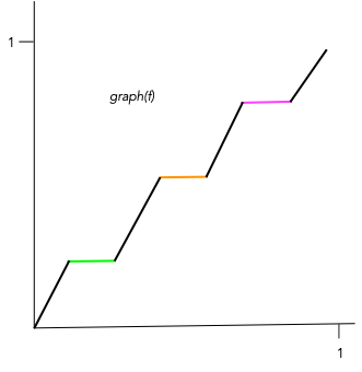
Recently Freedman gave me the fifteen second elevator proof of this Theorem. He drew a $1$-dimensional graph of $f$ with colored horizontal flats where $f$ is constant (see Figure 1). Then he applied a sort of inversion trick resulting in the graph of $g$, with lower length horizontal flats and vertical flats lying very close to the end points of the horizontal flats. Iterate this construction over and over to limit on a homeomorphism, noting that the lengths of the flats get smaller and smaller.
Note that to prove that $f$ is ABH, we pick an $\epsilon > 0$, shrink all the horizontal flats to length less than $\epsilon$ by a method moving no point more than $\epsilon /2$. Then repeat so that in going from the $k^{th}$ step to the $(k+1)^{st}$ step, no point is moved more than $\epsilon/s^k$, obtaining a homeomorphism which is within $\epsilon$ of $f$. This works for any $\epsilon$, so $f$ is ABH.

In November 2021, Bob Edwards described (on two sheets of paper) the argument that convinced him on Saturday, August 29, 1981 that Freedman did indeed have a proof of the four dimensional Poincare Conjecture, and much more.
I am writing here with a bit more detail what I learned from Mike and Bob.
I note that Mike’s Theorem has been generalized twice by Ric Ancel [1, 2], rewritten by Frank Quinn in [9], sketched well by Larry Siebenmann [14], and that recently Jeff Meier, Patrick Orson and Arumina Ray gave a proof in Chapter 9 of the grand exposition [3]. Danny Calegari has a description of the proof which is closest to the one here [5, page 26]. For a very sketchy outline of Mike’s argument see Chapter 13 of [13].
CASE 1 : ONE POINT
First we prove the Theorem in the case when $S_f$ consists of a single point $x \in B^n$ where $f^{-1} (x) = X$, see Figure 2. Given $\epsilon >0$ we can find a squeeze $\sigma : B^n \to B^n$ which by a homeomorphism takes $B^n$ onto the $\epsilon$-ball, $\epsilon B^n$, around $x$ and is the identity on $ \frac{\epsilon}{2} B^n$ around $x$.
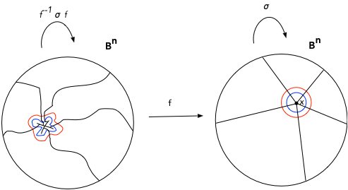
One non-trivial point inverse.
The map $f^{-1} \sigma f : B^n \to B^n$ (defined as the identity on $f^{-1} ( \frac{\epsilon}{2} B^n$) is the map which shrinks $f^{-1} (B^n)$ to
$f^{-1} (\epsilon B^n)$ while fixing $f^{-1} ( \frac{\epsilon}{2} B^n)$. With $f^{-1} \sigma f$, $f$ “conjugates” the usual coordinates on $B^n$ back to wiggly coordinates on $B^n$.
Now consider $\sigma f \sigma^{-1}$. This conjugation squeezes $f$ onto $\epsilon B^n$ keeping $ \frac{\epsilon}{2} B^n$ fixed pointwise.
Now define a homeomorphism $g:B^n \to B^n$ by setting $g = f^{-1} \sigma f \sigma^{-1}$ on $\epsilon B^n$; and $g=f^{-1}$ on $B^n – \epsilon B^n$. Then $g^{-1}\left(\frac{\epsilon}{2} B^n\right)$ approximates $f$, so, after iteration, $f$ is ABH.
CASE 2 : TWO POINTS
Now suppose $f$ has two points, $x$ and $y$, for which their inverses $X = f^{-1}(x)$ and $Y = f^{-1}(y)$ are non-trivial, see Figure 3. Define $\sigma_x$ as before (using the black rays), ignoring $y$, and similarly $\sigma_y$, ignoring $x$, and using the green rays. Now define the function $g$ piecewise based on the (red) $\epsilon$-balls $B^n_x$ and $B^n_y$ about $x$ and $y$ respectively.
Let $g=f^{-1} \sigma_x f \sigma^{-1}_x$ on $\epsilon B^n_x$; let $g=f^{-1} \sigma_y f \sigma^{-1}_y$ on $\epsilon B^n_y$; and let $g=f^{-1}$ elsewhere.
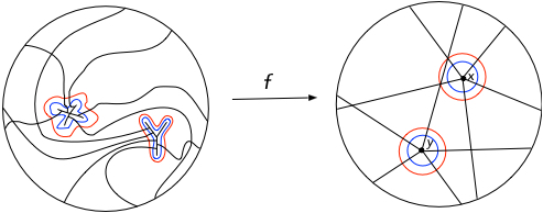
Two non-trivial point inverses, X and Y.
Note that $g$ is no longer a homeomorphism because $Y$ is now found in $\epsilon B^n_x -\frac{\epsilon}{2}B^n_x$ for observe that $\sigma_x f \sigma_x^{-1}$ squeezes $f$ into $\epsilon B_x$ which now contains both singular points, and then composing with $f^{-1}$ only allows the removal of $x$, leaving $y$, see Figure 3. Similarly with $x$ remaining a singular point.
It appears we have made no progress for there are still two singular points, but their point inverses now lie in $\epsilon$-balls. If we iterate this process, we find the point inverses (the horizontal and vertical flats in Freedman’s sketch) lie in smaller and smaller $n$-balls, so that the limit is a homeomorphism. Thus $f$ is ABH.
CASE 3 : THREE POINTS
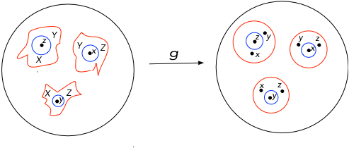
Now we assume that $S_f$ is three points, $x, y,$ and $z$. We perform the same constructions using three squeezes, $\sigma_x, \sigma_y$ and $\sigma_z$. We end up with a $g$ that has six non trivial point inverses, and they lie in the $\epsilon$-balls, but outside the $\epsilon/2$-balls, as shown in Figure 4. The key fact is that they lie in $\epsilon$-balls, so we iterate the construction, producing at the $k^{th}$ step $k(k-1)$ non-trivial point inverses, all lying in $\epsilon/k$ balls, thus limiting to a homeomorphism. This finishes the proof if $S_f$ is finite. (Note that $X, Y$ and $Z $ play the role of the three colors in Mike’s quick sketch in Section 3.)
INFINITELY-MANY NONTRIVIAL POINT INVERSES
The key to the proof when $S_f$ is not finite is a condition that there are only a finite number of point inverses which have volume bigger than a given $\epsilon$, as well as a condition that allows us to choose red $\epsilon$-balls and blue $\epsilon/2$-balls whose boundaries are disjoint from $S_f$. The first is implied by the null condition. The second is implied by the definition of tame.
Now the proof proceeds exactly as in the case when $S_f$ is finite. At the $k^{th}$ stage we define $g$ as before, with the result that instead of $k(k-1)$ non-trivial point inverses, each with volume less than $\epsilon/{2^k}$, we have infinitely many non-trivial point inverses but still having volume less than $\epsilon/{2^k}$. In the limit all point inverses have shrunk to points and we have a homeomorphism. Thus $f$ is ABH.
BACKGROUND
In Spring 1974, Bob Edwards and I were visiting IHES. Andrew Casson came over from Cambridge (UK) and gave two spectacular lecture series [12]. One was on the Casson-Gordon invariant of knots and does not concern us here. The other presented his partial solution to the problem of embedding $2$-handles into a $4$-manifold $X$ when algebraic data called for them.
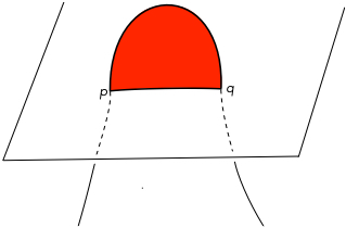
If a circle $C$ is embedded in $X$ and is homotopically trivial, then we would like to fill in $C$ with an embedded disk, a $2$-handle, but it may only be possible to immerse the disk. The double points of this immersion can come in pairs which we try to eliminate by use of Whitney disks (see Figure 5 ) where by pulling the arc across the red Whitney disk, the pair of double points disappear. The problem is that the Whitney disk may have double points. Casson’s great idea was to proceed by finding Whitney disks for the double points in the first stage of Whitney disks. Of course the second stage Whitney disks might also have double points, as might the third stage Whitney disks, and so on. This infinite construction (of thickened disks) produced a proper homotopy $2$-handle. Casson called these flexible handles, but they quickly became known as Casson handles.
Casson also knew that each of these Casson handles was the complement of a cone on a generalized Whitehead continuum in $B^2 \times S^1 \subset B^2 \times B^2$.
All this is described in my favorite (since I wrote it 40 years ago) reference [13, Chapter 12].
I returned to Berkeley with eight pages of notes on Casson’s lectures and gave a copy to Mike; seven years later, after tutelage by Bob on decomposition spaces, Mike had his stunning results including the topological four dimensional Poincare Conjecture. Even more surprising, six months later, was the existence of exotic smooth structures on $R^4$ which could have been an addendum to Donaldson’s paper [6] coauthored by Simon himself and Freedman and Edwards. As it is, there is no paper giving the first exotic $R^4$, but there is for the second and third[11] and also [13. Chapter 14].
Returning to Casson handles, Bob thought of proceeding by examining the outside of a Casson handle as it lay naturally in $B^2 \times B^2$, but Mike chose instead to investigate the inside of a Casson handle, $CH_*$.
Mike explored $CH_*$ by embedding a “design” of (capped) Casson handles in $CH_*$, and then collapsing the unexplored regions to points, thereby finding a quotient map $CH_* \to V$ [13, Chapter 13].
A classical Bing shrinking type argument showed that $V$ was homeomorphic to $B^2 \times R^2$. Then extending by the identity to $S^4$,
\[ S^4 \supset B^2 \times R^2 \supset CH_* \to V \subset S^4 ,\]
we apply Mike’s hard decomposition theorem to conclude that
$$CH_* = B^2\times R^2 .$$
MORE BACKGROUND
Why is Mike’s hard decomposition theorem necessary, why not a classical decomposition argument? Recall Bing’s proof [4] that the union of two exteriors of Alexander’s horned balls, $\Sigma^3$, is homeomorphic by $\phi$ to $S^3$. This is done, as are later decomposition proofs, by approximating $\phi$ by diffeomorphisms; all the steps are done smoothly as in Step 1 above. We leave the world of diffeomorphisms already in Step 2.
It was observed in 1974, (see Bob’s Remark on page 234 of [12] that if the decompositions used to understand Casson handles could be approximated by diffeomorphisms, then certain links would be smoothly slice, which seemed unlikely at the time. When Donaldson’s work appeared in early 1982, (showing that these links were not smoothly slice,) it was clear to those few who were aware of Bob’s Remark that Casson’s decompositions could not be approximated by diffeomorphisms, and thus a new idea, the hard version, was necessary.
It is worth mentioning a very recent work [10] of Mike and Mike Starbird concerning the homeomorphism $\phi$ from $\Sigma$ to $S^3$, and its modulus of continuity, MOC (see Wikipedia).
The two Mikes prove that the MOC for $\phi$ is sub-exponential. Moreover, given any monotonically increasing continuous function, they can find a more complicated decomposition of a different $\Sigma$ (there are many versions of the Alexander horned sphere) whose $\phi$ has a larger MOC. These $\phi$, although approximable by diffeomorphisms, are nonetheless very wild.
BIBLIOGRAPHY
[1] Ancel, Frederic, Approximating cell-like maps of S4 by homeomorphisms, Con- temporary Mathematics 35 (1984), 143-164.
[2] Ancel, Frederic, Recursively squeezable sets are squeezable,- https://arxiv.org/pdf/2009.02817.pdf
[3] Behrens, Stefan; Boldiz ́ar, Kalm ́ar; Kim, Min Hoon; Powell, Mark; and Ray Arumina, The Disc Embedding Theorem, Oxford Univ. Press, 2021, xiv+473.
[4] Bing, R. H. A homeomorphism between the 3-sphere and the sum of two solid horned spheres. Annals of Mathematics, 52 (1952), 354–362.
5] Calegari, Danny math.uchicago.edu\/~dannyc/books\/4dpoincare\ /4dpoincare.html
[6] Donaldson, Simon K. An application of gauge theory to four-dimensional topol- ogy. Journal of Differential Geometry, 18 (1983), 279–315.
[7] Edwards, Robert D. The Topology of Manifolds and Cell-Like Maps., Proc. Int. Congress Math, Helsinki 1978, Acad. Sci. Fennica, Helsinki, 1980, 111-127.
[8] Freedman, M. H., The topology of $4$-dimensional manifolds. J. Diff. Geom., 17 (1982), 357–453.
[9] Freedman, Michael H., and Quinn, Frank, Topology of $4$-Manifolds, Princeton Univ. Press,, Princeton Math. Series V39, 1990.
[10] Freedman, Michael and Starbird, Michael, The geometry of the Bing involution, To appear.
[11] Gompf, Robert. Three exotic $\mathbf{R}^4$’s and other anomalies J. Differential Geom. 18, (1983), 317-328.
[12] Guillou, Lucien and Marin, Alexis A la Recherche de la Topologie Perdue, Birkhauser, 1986, iv + 244.
[13] Kirby, Robion C., The topology of $4$-manifolds, Lecture Notes in Mathematics}, v. 1374, Springer-Verlag, Berlin, 1989, vi+108.
[14] Siebenmann, Laurent, La conjecture de Poincare topologique en dimension $4$, Seminaire Bourbaki, 24, (1981-82), Soc. Math. France, 219-248.
.
Related Videos
Michael Freedman, A personal story of the 4D Poincare conjecture, Youtube video., 2021.
Bob Edwards History of Michael Freedman’s Proof of the 4-d Poincare Conjecture, Youtube video from the Freedman 60 workshop, 6/21/2011/