AUTHOR : C. Adams :
EDITOR/ART : R. Ghrist :
To move mathematics forward, researchers are constantly seeking new relationships between various areas of mathematics. The farther apart two areas are, the more dramatic the implications when relationships are discovered. But how to find these relationships? Certainly, studying the fields and developing intuition plays a critical role. But there is also the option of generating lots of data and searching for patterns in the data. Once a suspected relationship is uncovered, mathematicians can then try to prove that the result holds.
But rather than just combing through data, researchers have now begun to apply artificial intelligence techniques to predict connections and to search for mathematical objects with particular properties. In this review, we consider six recent papers that apply neural networks to questions from knot theory.
A neural network can be thought of as an adjustable function $f$ that is defined on a dataset $D \subset \mathbb{R}^n$, taking values in, say, a set $S \subset \mathbb{R}^m$. Taking a subset of $D$ for which the desired values of $f$ are known, we train the network to approximately and efficiently try to match those values. It is then applied to a broader subset of $D$ for which its values are known to validate its prediction capabilities. Once satisfied, we can then run it on those elements of $D$ for which we do not know the values. Unlike some statistical methods, the function is far from being linear.
To generate such a function, we first choose an architecture for the neural network with parameters that can be tuned via the training set. But we do not want to overfit the data, so we limit the number of parameters we can adjust.

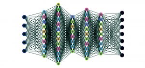
For instance, as in the figure above, we might start with an input layer, five hidden layers and an output layer. In our case, the input might be knots formatted in a particular manner, for instance as a Gauss code representation of a knot diagram, or as a cycle of vertices in 3-space with adjacent vertices connected by straight line segments, or as a permutation of integers obtained from a petal representation of a knot. Or the input could be a set of particular choices for invariants associated to the knot. The output might be types of knots or other invariants for the knots. Each edge has a weight associated to it that can be adjusted.
Neural networks can be substantially more complicated, but for our purposes, this model suffices. For more background on the subject of neural networks, a good introduction is the video series by 3Blue1Brown.
In [3], which we will discuss in more detail shortly, the authors provide a simple example to help motivate the idea. Suppose we take as input quantities we can calculate from a convex polyhedron. For instance, we might take as input a vector with entries the number of vertices, the number of edges, the surface area and the volume. Now suppose we would like to find a relationship between this input data and the number of faces of the polyhedron. By training the neural network on large numbers of convex polyhedra, it may converge on the simple solution that the first entry minus the second entry of the input vector is equal to 2 minus the number of faces. In other words, it rediscovers Euler’s Theorem. Of course, we already knew Euler’s Theorem, but if we had not, this would have pointed us to the conjecture and then we would have been motivated to prove it.
In A neural network approach to computing knot invariants, the author applies neural networks to help in the search for knots that are quasipositive [6], meaning that it can be represented by a braid generated by a product of conjugations of positive crossings. A quasipositive representative of a knot is useful in that in [10], Rudolph showed that one could use it to directly determine the slice genus $g_4(K)$ of the knot $K$. Further, for quasipositive knots, the $\tau$-invariant of Ozsváth and Szabó, defined in terms of the Heegaard-Floer homology, is equal to the slice genus $g_4(K)$. So there are very good reasons to want to know whether a knot is quasipositive and to determine a quasipositive braid representation if it is. Once trained on a subset of the knots, the network achieves a success rate in identifying quasipositive knots from blind validation sets of greater than 99.93% . It also determines $g_4(K)$ and $\tau(K)$ with mean validation accuracies of 93.70% and 99.97% respectively. Considering 179 knots of twelve or fewer crossings for which quasipositivity had not been determined, the methods pointed to additional candidates which could then be verified and resulted in the determination of 84 new quasipositive knots.
As the author points out, there are limitations to the neural network approach. Although they can point toward a relationship, in no way do they constitute a proof. Furthermore, however effective a neural network is at prediction, they are often at present a black box. It is difficult to deduce from where that effectiveness comes. Moreover, one should also be careful about how the training set, which consists of knots for which particular invariants are known, may differ from the broader class of knots. The metaphorical floor of knot theory is littered with conjectures posited on relatively simple collections of knots for which counterexamples appeared when more complicated knots were considered.
Another opportunity to apply neural networks is to look for relationships between various invariants associated to a knot. In Advancing Mathematics by Guiding Human Intuition with AI, the authors describe an application of neural networks to finding correlations between algebraic and geometric invariants of knots [3].
The signature of a knot is an invariant that was first defined by Trotter in 1962. It is an even integer computed from the Seifert module of the knot. It is an algebraic invariant in that it comes out of the homology associated to the knot complement and its spanning surface. On the other hand, there are also geometric invariants of knots. In the 1980’s, William Thurston showed that all knots fall into three categories: torus knots that sit on the surface of an unknotted torus, satellite knots that live in a toroidal fattening of another knot, and hyperbolic knots, which have a metric of constant curvature -1 on their complements. The Mostow-Prasad Rigidity Theorem tells us that for hyperbolic knots, this metric is unique and hence any measurable quantities that come out of this metric are invariants useful for distinguishing knots.
We would like to find relationships between the algebraic invariants and the geometric invariants of knots. There are many invariants known to have algebraic or combinatorial definitions that as of yet have no known connection to the geometric structure on the knot complement. A huge step in this direction would be to prove the Volume Conjecture, formulated by Rinat Kashaev in 1997. Since then, it has been proved for a handful of knots. It posits a relationship between the hyperbolic volume of a knot and the asymptotic behavior of the colored Jones polynomial, another algebraic invariant. Specifically,
$\displaystyle \lim_{ N \to \infty} \frac{2\pi \ln |J_{K,N} (e^{2\pi i})|}{N} = \text{Vol}(K)$
where the colored Jones polynomial $ J_{K,N} (q)$ can be defined in terms of the Jones polynomials of parallel copies of the knot $K$.
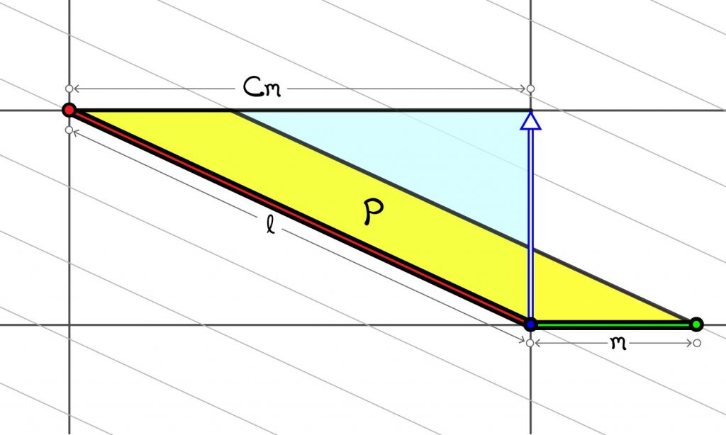
But there are a variety of invariants other than volume that come out of the metric on a hyperbolic knot. In particular, one can look at the geometry of the cusp. The cusp is a neighborhood of the missing knot in the complement of the knot. For a hyperbolic knot, the boundary of the cusp is a torus with a Euclidean 2-dimensional metric. A fundamental domain for this cusp boundary is a parallelogram $P$ in the Euclidean plane with one boundary corresponding to the meridian of the knot and the other boundary corresponding to the longitude. If we fire a geodesic ray from their intersection that is perpendicular to the meridian, it will wrap around the cusp torus and hit the meridian again. The number $C$ of meridians away from its initial point on the meridian, which need not be a whole number, is the natural slope of the cusp boundary. In the Euclidean plane, we see the natural slope as in the figure below.

This is not an invariant that has been considered previously. But in the neural network from [3], it turns out to have the best correlation with the signature. The relationship between the invariants suggested by the neural network was subsequently proved in [2]. So this is an excellent example of how neural networks can point to conjectures that can then be proved.
The Volume Conjecture considers the relationship between the asymptotic behavior of the colored Jones polynomial of a hyperbolic knot and its hyperbolic volume. In Deep learning the hyperbolic volume of a knot, the authors sought to find a direct connection between the Jones polynomial and the hyperbolic volume of knots [5]. They utilized a neural network with two hidden layers of 100 neurons each that was able to yield surprisingly accurate volume estimates for knots from the Jones polynomials of the knots. The results suggest that a nonlinear equation (like the one above) may also hold for the Jones polynomial itself, perhaps with some adjustment terms from other invariants.
In Learning knot invariants across dimensions, the authors investigate correlations between the invariants given by the Jones polynomial $J_K(q)$, the Khovanov polynomial $\text{Kh}(q, t)$, the smooth slice genus $g_4(K)$, and Rasmussen’s $s$-invariant [1].
For this purpose, they employ two different methods to generate random knots. The first uses the fact that every knot is represented by a braid, and so one can randomize by generating random braid words. The second uses the fact that every knot can be put into a petal diagram which is represented by a permutation on integers. So one can then use this to generate random knots via random permutations as in [5].
Although their trained neural network predicts $s$ with 99% accuracy from $\text{Kh}(q,-q^{-4})$, this is a good example of the limitations inherent in such techniques. A theoretical explanation for the correlation is the so-called Knight Move Conjecture on Khovanov homology. It has been proved for all alternating knots, all quasialternating knots and all knots of unknotting number two or less and in fact held for all of the knots in the dataset, but it was disproved in 2018 [9] with a counterexample of 38 crossings.
On the other hand, the authors of [1] also find similar relations between $s$ and $\text{Kh}(q,-q^{-2})$; between $g_4$ and $\text{Kh}(q,t)$; and realize 95% accuracy in predicting $g_4$ and $s$ from $J_K(q)$. These correlations present interesting opportunities to pursue connections between these invariants.
Neural networks have been applied to the oldest problem in knot theory: how do you identify a particular knot from a representation? In Identifying knot types of polymer conformations by machine learning, the authors represent knots as polymers in the sense of equal-length rods glued end-to-end [11]. They take representatives of the five simplest knots, including the trivial knot, $3_1$, $4_1$, $5_1$ and $5_2$, and then train various architectures of neural networks to try to determine the knot type of a given representative. Their best model achieves a 99% success rate on polymers consisting of 100 rods.
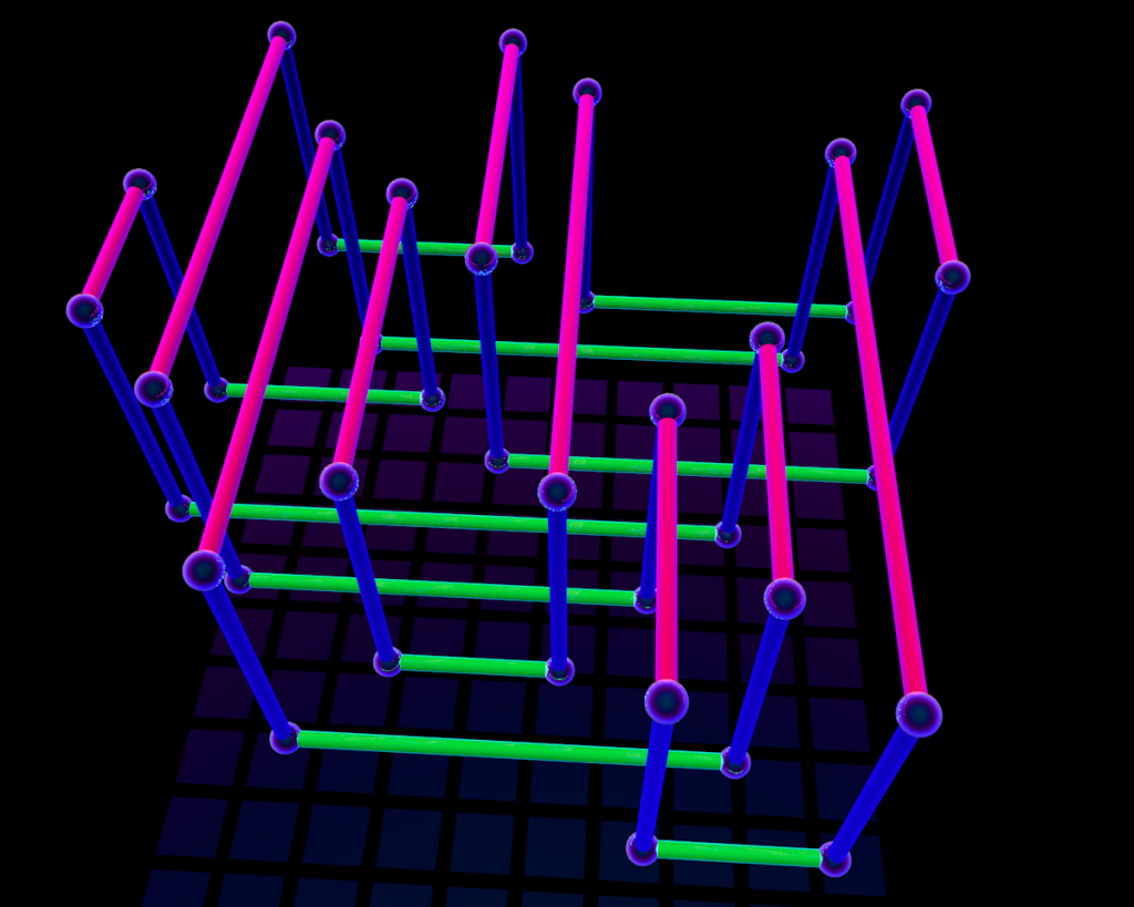
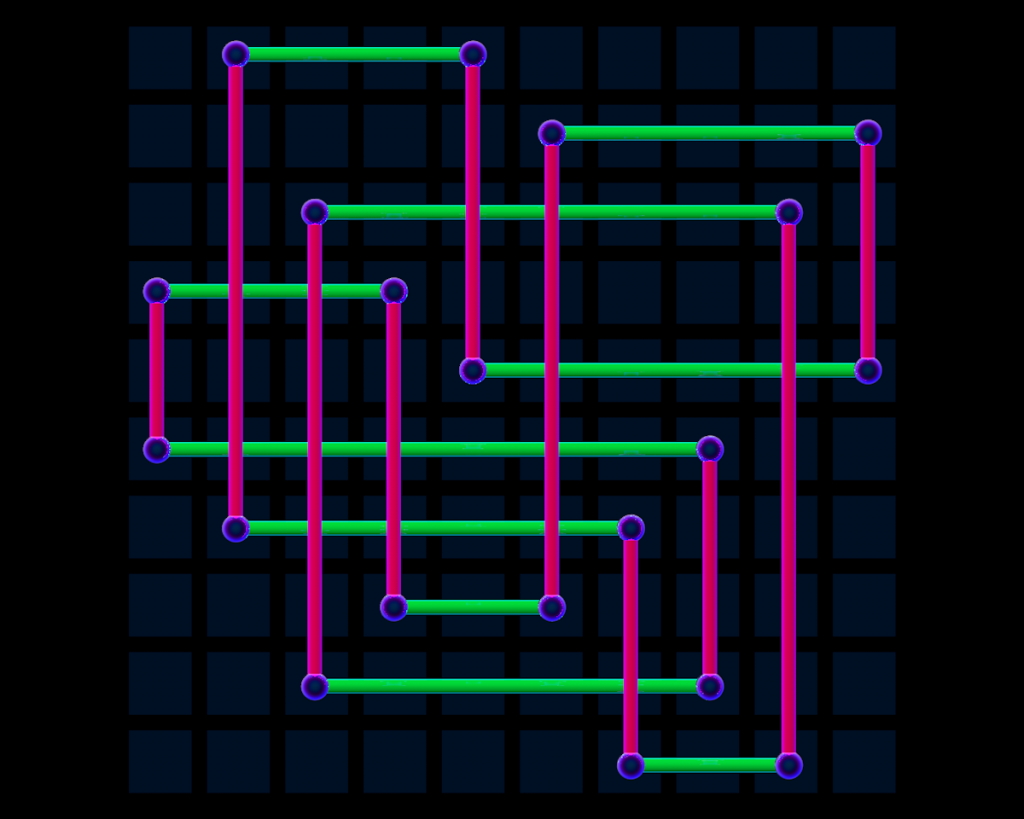
The preprint Rectangular knot diagrams classification with deep learning considers the same problem [8]. This relies on results of I. Dynnikov [4], who provided an algorithm that starts with a knot in a special rectangular form (see figure below). In this form, there is a projection to a square planar grid, in which each row [column] has exactly one horizontal [vertical] edge, and where each vertical edge crosses over the horizontal edges. It is straightforward to represent such a diagram via an $n \times 2$ matrix, where $n$ is the number of horizontal [equivalently, vertical] edges: this is the complexity of the diagram. Dynnikov showed that if the knot is trivial, there must be a sequence of monotonically simplifying moves, now called Dynnikov moves, that will reduce it to a trivial projection [4].


In [8], the authors generate their own data by starting with simple rectangular knot diagrams for the 36 knots of eight or fewer crossings, and then complicate them by applying Dynnikov moves. They then train their neural network to identify which type of knot a given diagram represents. Once trained, the neural network achieved a correct identification of knots that were trivial 84% of the time. For other types of knots, it is less successful. For instance, it correctly identifies the knot $5_1$ only 34% of the time, often confusing it with the other two-braid knots $3_1$ and $7_1$.
The model is much more successful when only certain (“internal”) Dynnikov moves are used to complicate the original rectangular diagrams. And interestingly, sometimes the neural network is better at identifying diagrams with higher complexity than with lower complexity. Further research will seek to understand these phenomena and to use neural networks to determine possible sequences of Dynnikov moves to simplify diagrams.
Clearly, neural networks have a contribution to make in knot theory and more generally across mathematics. They can point us to potential theorems, conjectures, and algorithms and they can help to identify mathematical objects with certain properties. This area provides an opportunity for very fruitful collaboration between the artificial intelligence and the mathematics communities that could have a substantial impact as we move forward.
BIBLIOGRAPHY
[1] J. Craven, M. Hughes, V. Jejjala, and A. Kar. Learning knot invariants across dimensions. ArXiv:2112.00016. SciPost Phys. 14 (2023), no. 2, Paper No. 021, 28 pp.
[2] A. Davies, M. Lackenby, A. Juhasz, and N. Tomašev. The signature and cusp geometry of hyperbolic knots. ArXiv:2111.15323.
[3] A. Davies, P. Veličković, L. Buesing, et al. Advancing mathematics by guiding human intuition with AI. Nature, 600 (2021), 70–74.
[4] I. Dynnikov. Arc-presentations of links: monotonic simplification. Fund. Math., 190 (2006), 29–76.
[5] C. Even-Zohar, J. Hass, N. Linial, and T. Nowik. The distribution of knots in the petaluma model. Algebraic and Geometric Topology], 18 (2018), 3647–3667.
[6] M. Hughes. A neural network approach to predicting and computing knot invariants. J. of Knot Thy. and its Ram., 29(3) (2020), 2050005.
[7] V. Jejjala, A. Kar, and O. Parrikar. Deep learning the hyperbolic volume of a knot. ArXiv:1902.05547. Phys. Lett. B 799 (2019), 135033, 7 pp.
[8] L. Kauffman, N. Russkikh, and I. Taimanov. Rectangular knot diagrams classification with deep learning. ArXiv:2011.03498. J. Knot Theory Ramifications 31 (2022), no. 11, Paper No. 2250067, 20 pp.
[9] C. Manolescu and M. Marengon. The knight move conjecture is false. Proc. Amer. Math. Soc., 148 (2020), 435–439.
[10] L. Rudolph. Quasipositivity as an obstruction to sliceness. Bulletin Amer. Math. Soc., 29(1) (1993), 51–59.
[11] O. Vandans, K. Yang, Z. Wu, and L. Dai. Identifying knot types of polymer conformations by machine learning. Phys. Rev. E], 101 (2020), 022502.
.

